You can download this guide as a Jupyter notebook.

Working with xarray

rigid_body_motion provides first class support for xarray data types. xarray has several features that make working with motion data convenient:

1. xarray is designed to combine physical data with metadata such as timestamps.

2. xarray’s Dataset class can be used as a container for timestamped transformations.

3. Arbitrary metadata can be attached to arrays to keep track of e.g. reference frames.

We recommend you to familiarize yourself with xarray before working through this tutorial. Their documentation is an excellent resource for that.

Note

The following examples require the matplotlib, xarray and netcdf4 libraries.

import rigid_body_motion as rbm
import xarray as xr
import matplotlib.pyplot as plt

plt.rcParams["figure.figsize"] = (10, 5)

Loading example data

rigid_body_motion includes a recording of head and eye tracking data (using the Intel RealSense T265 as the head tracker and the Pupil Core eye tracker). This data can be loaded with xr.open_dataset:

head = xr.open_dataset(rbm.example_data["head"])
head

Downloading data from 'https://github.com/phausamann/rbm-data/raw/main/head.nc' to file '/home/docs/.cache/pooch/58826f066ba31bf878bd1aeb5305d7d4-head.nc'.

<xarray.Dataset> Size: 8MB
Dimensions:           (time: 66629, cartesian_axis: 3, quaternion_axis: 4)
Coordinates:
  * time              (time) datetime64[ns] 533kB 2020-02-02T00:27:14.3003652...
  * cartesian_axis    (cartesian_axis) <U1 12B 'x' 'y' 'z'
  * quaternion_axis   (quaternion_axis) <U1 16B 'w' 'x' 'y' 'z'
Data variables:
    position          (time, cartesian_axis) float64 2MB ...
    linear_velocity   (time, cartesian_axis) float64 2MB ...
    angular_velocity  (time, cartesian_axis) float64 2MB ...
    confidence        (time) float64 533kB ...
    orientation       (time, quaternion_axis) float64 2MB ...

xarray.Dataset

• Dimensions:
  • time: 66629
  • cartesian_axis: 3
  • quaternion_axis: 4
• Coordinates: (3)
  • time
    (time)
    datetime64[ns]
    2020-02-02T00:27:14.300365210 .....

    long_name :

    Time

    array(['2020-02-02T00:27:14.300365210', '2020-02-02T00:27:14.305364370',
           '2020-02-02T00:27:14.310361385', ..., '2020-02-02T00:32:47.283535480',
           '2020-02-02T00:32:47.288533449', '2020-02-02T00:32:47.293531418'],
          dtype='datetime64[ns]')

  • cartesian_axis
    (cartesian_axis)
    <U1
    'x' 'y' 'z'

    long_name :

    Axis

    array(['x', 'y', 'z'], dtype='<U1')

  • quaternion_axis
    (quaternion_axis)
    <U1
    'w' 'x' 'y' 'z'

    long_name :

    Axis

    array(['w', 'x', 'y', 'z'], dtype='<U1')

• Data variables: (5)
  • position
    (time, cartesian_axis)
    float64
    ...

    long_name :

    Position

    units :

    m

    [199887 values with dtype=float64]

  • linear_velocity
    (time, cartesian_axis)
    float64
    ...

    long_name :

    Linear velocity

    units :

    m/s

    [199887 values with dtype=float64]

  • angular_velocity
    (time, cartesian_axis)
    float64
    ...

    long_name :

    Angular velocity

    units :

    rad/s

    [199887 values with dtype=float64]

  • confidence
    (time)
    float64
    ...

    [66629 values with dtype=float64]

  • orientation
    (time, quaternion_axis)
    float64
    ...

    long_name :

    Orientation

    [266516 values with dtype=float64]

• Indexes: (3)
  • time
    PandasIndex

    PandasIndex(DatetimeIndex(['2020-02-02 00:27:14.300365210',
                   '2020-02-02 00:27:14.305364370',
                   '2020-02-02 00:27:14.310361385',
                   '2020-02-02 00:27:14.315360308',
                   '2020-02-02 00:27:14.320358515',
                   '2020-02-02 00:27:14.325356245',
                   '2020-02-02 00:27:14.330354452',
                   '2020-02-02 00:27:14.335352182',
                   '2020-02-02 00:27:14.340350628',
                   '2020-02-02 00:27:14.345348358',
                   ...
                   '2020-02-02 00:32:47.248551607',
                   '2020-02-02 00:32:47.253549576',
                   '2020-02-02 00:32:47.258547305',
                   '2020-02-02 00:32:47.263544559',
                   '2020-02-02 00:32:47.268542528',
                   '2020-02-02 00:32:47.273540258',
                   '2020-02-02 00:32:47.278538465',
                   '2020-02-02 00:32:47.283535480',
                   '2020-02-02 00:32:47.288533449',
                   '2020-02-02 00:32:47.293531418'],
                  dtype='datetime64[ns]', name='time', length=66629, freq=None))

  • cartesian_axis
    PandasIndex

    PandasIndex(Index(['x', 'y', 'z'], dtype='object', name='cartesian_axis'))

  • quaternion_axis
    PandasIndex

    PandasIndex(Index(['w', 'x', 'y', 'z'], dtype='object', name='quaternion_axis'))

• Attributes: (0)

The dataset includes position and orientation as well as angular and linear velocity of the tracker. Additionally, it includes the physical dimensions time, cartesian_axis (for position and velocities) and quaternion_axis (for orientation). Let’s have a look at the position data:

head.position

<xarray.DataArray 'position' (time: 66629, cartesian_axis: 3)> Size: 2MB
[199887 values with dtype=float64]
Coordinates:
  * time            (time) datetime64[ns] 533kB 2020-02-02T00:27:14.300365210...
  * cartesian_axis  (cartesian_axis) <U1 12B 'x' 'y' 'z'
Attributes:
    long_name:  Position
    units:      m

xarray.DataArray

'position'

• time: 66629
• cartesian_axis: 3

• ...

  [199887 values with dtype=float64]

• Coordinates: (2)
  • time
    (time)
    datetime64[ns]
    2020-02-02T00:27:14.300365210 .....

    long_name :

    Time

    array(['2020-02-02T00:27:14.300365210', '2020-02-02T00:27:14.305364370',
           '2020-02-02T00:27:14.310361385', ..., '2020-02-02T00:32:47.283535480',
           '2020-02-02T00:32:47.288533449', '2020-02-02T00:32:47.293531418'],
          dtype='datetime64[ns]')

  • cartesian_axis
    (cartesian_axis)
    <U1
    'x' 'y' 'z'

    long_name :

    Axis

    array(['x', 'y', 'z'], dtype='<U1')

• Indexes: (2)
  • time
    PandasIndex

    PandasIndex(DatetimeIndex(['2020-02-02 00:27:14.300365210',
                   '2020-02-02 00:27:14.305364370',
                   '2020-02-02 00:27:14.310361385',
                   '2020-02-02 00:27:14.315360308',
                   '2020-02-02 00:27:14.320358515',
                   '2020-02-02 00:27:14.325356245',
                   '2020-02-02 00:27:14.330354452',
                   '2020-02-02 00:27:14.335352182',
                   '2020-02-02 00:27:14.340350628',
                   '2020-02-02 00:27:14.345348358',
                   ...
                   '2020-02-02 00:32:47.248551607',
                   '2020-02-02 00:32:47.253549576',
                   '2020-02-02 00:32:47.258547305',
                   '2020-02-02 00:32:47.263544559',
                   '2020-02-02 00:32:47.268542528',
                   '2020-02-02 00:32:47.273540258',
                   '2020-02-02 00:32:47.278538465',
                   '2020-02-02 00:32:47.283535480',
                   '2020-02-02 00:32:47.288533449',
                   '2020-02-02 00:32:47.293531418'],
                  dtype='datetime64[ns]', name='time', length=66629, freq=None))

  • cartesian_axis
    PandasIndex

    PandasIndex(Index(['x', 'y', 'z'], dtype='object', name='cartesian_axis'))

• Attributes: (2)

  long_name :

  Position

  units :

  m

As you can see, this is a two-dimensional array (called DataArray in xarray) with timestamps and explicit names for the physical axes in cartesian coordinates.

xarray also provides a straightforward way of plotting:

head.linear_velocity.plot.line(x="time")

[<matplotlib.lines.Line2D at 0x7970f6b39ff0>,
 <matplotlib.lines.Line2D at 0x7970f6b686a0>,
 <matplotlib.lines.Line2D at 0x7970f6b68670>]

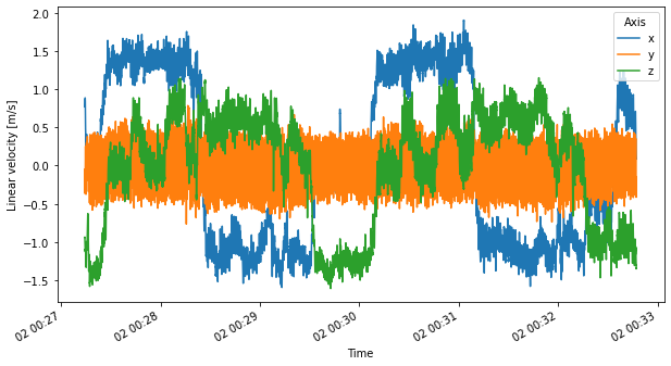
The example recording is from a test subject wearing the combined head/eye tracker while walking twice around a building. The head tracking data is represented in a world-fixed reference frame whose origin is at the head tracker’s location at the start of the recording.

In the next step, we will leverage rigid_body_motion’s powerful reference frame mechanism to transform the linear velocity from world to tracker coordinates.

Reference frame interface

As in the previous tutorial, we begin by registering the world frame as root of the reference frame tree:

rbm.register_frame("world")

Timestamped reference frames can be easily constructed from Dataset instances with the ReferenceFrame.from_dataset() method. We need to specify the variables representing translation and rotation of the reference frame as well as the name of the coordinate containing timestamps and the parent frame:

rf_head = rbm.ReferenceFrame.from_dataset(
    head, "position", "orientation", "time", parent="world", name="head"
)

Let’s register this reference frame so that we can use it easily for transformations:

rf_head.register()

Now we can use transform_linear_velocity() to transform the linear velocity to be represented in tracker coordinates:

v_head = rbm.transform_linear_velocity(
    head.linear_velocity, outof="world", into="head", what="representation_frame"
)
v_head.plot.line(x="time")

[<matplotlib.lines.Line2D at 0x7970f5ffbf40>,
 <matplotlib.lines.Line2D at 0x7970f5ffae30>,
 <matplotlib.lines.Line2D at 0x7970f5e28190>]

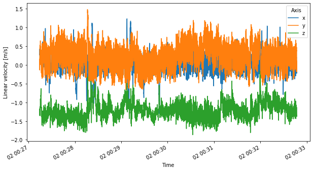
We now see a mean linear velocity of ~1.4 m/s in the negative z direction. This is due to the coordinate system defined by the RealSense T265 where the positive z direction is defined towards the back of the device.